基础结构
RNN基础单元:
在RNN基础单元中,隐藏层状态由输入层和上一时刻的状态决定,即隐藏层的计算是$X_tW_{xh} + H_{t-1}W_{hh}$ ,而这个计算可以通过将$X_t$与$H_{t-1}$连结后的矩阵与$W_{xh}$与$W_{hh}$连结后的矩阵相乘得到。
1 | import torch |
这两种方法得到的结果都是一样的。
梯度计算
以时间序列为3的计算图为例:
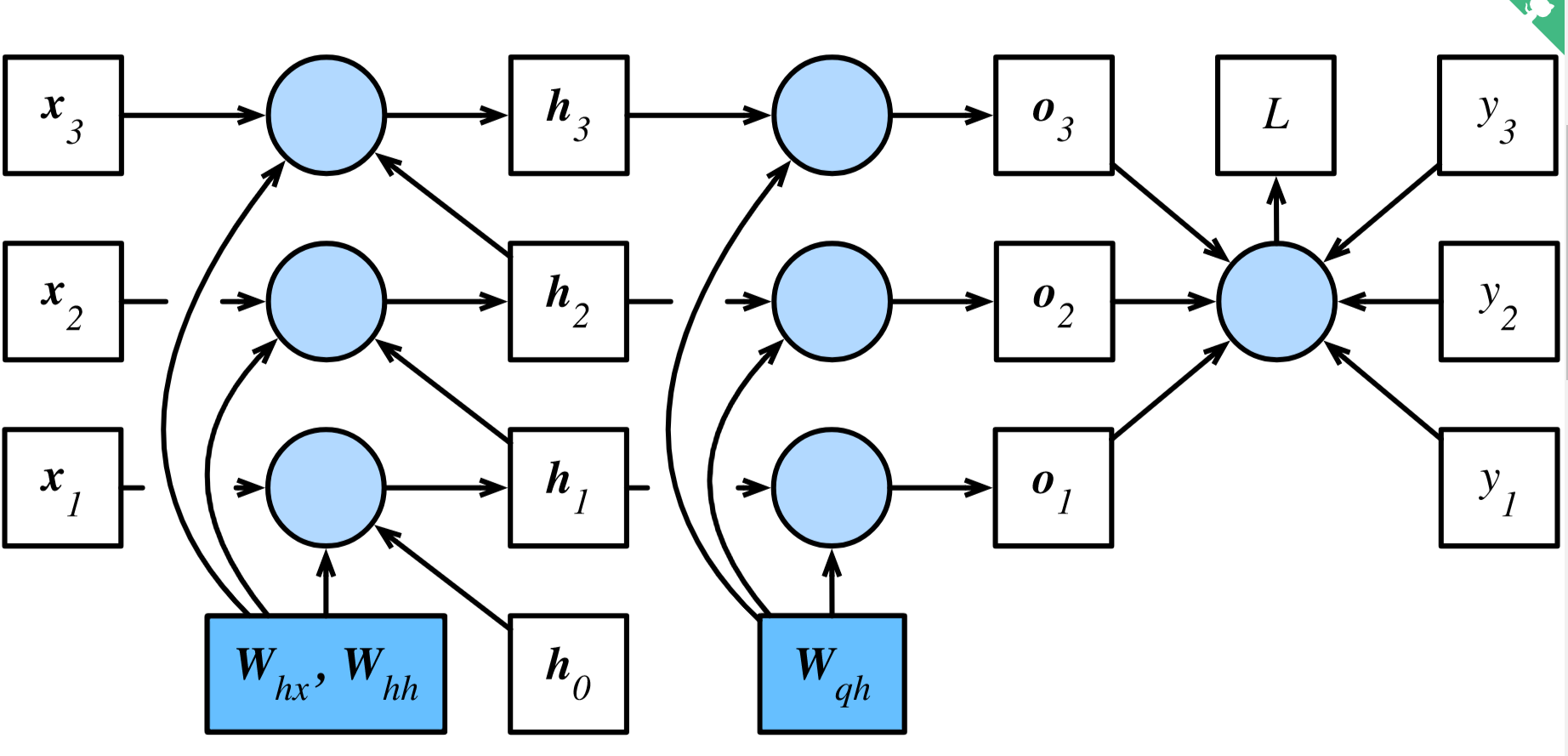
其前向计算公式为:
从L开始倒推梯度:
输出层参数:(sum是因为共享参数,乘积是链式法则)
在计算隐藏层参数$W_{hh}$ 时,它们通过隐藏层状态$h_t$产生了依赖关系。因此先计算最终时间步T的$h_T$的梯度:
而对于$t < T$的情况,需要从后往前计算,这样对于每个$h_t$的梯度在计算时,后面依赖它的$h$的梯度都被计算出了。则根据链式求导法则$h_t$的梯度包含$o_t$和之后的$h$ 对$h_t$的偏导。于是这变成了一个关于$h_t$的递推式:
由上式中的指数项可见,当$T$与$t$之差较大时,容易出现梯度衰减和爆炸。而$h_t$的梯度也会影响其他参数的梯度,比如$W_{hh}、W_{hx}$ ,它们在隐藏层间共享参数,$h_1, \cdots, h_T$都依赖它们,因此:
读取数据集
1 | import torch |
采样时序数据
- 随机采样
下面的代码每次从数据里随机采样一个小批量。其中批量大小batch_size指每个小批量的样本数,num_steps为每个样本所包含的时间步数(一个时间序列)。 在随机采样中,每个样本是原始序列上任意截取的一段序列。相邻的两个随机小批量在原始序列上的位置不一定相毗邻。因此,我们无法用一个小批量最终时间步的隐藏状态来初始化下一个小批量的隐藏状态。在训练模型时,每次随机采样前都需要重新初始化隐藏状态。
1 | # 参数包含语料索引,批量大小,每个样本的序列长度 |
- 相邻采样
注意相邻采样是在连续的epoch之间相邻,若一个epoch中有多个batch_size,则不同batch之间的样本不一定连续。因此可将样本按batch_size分割,再依次按epoch顺序取。
1 | # |
基础RNN
手动实现
1 | import time |
torch函数实现
1 | num_hiddens , num_steps, batch_size= 256, 35, 2 |
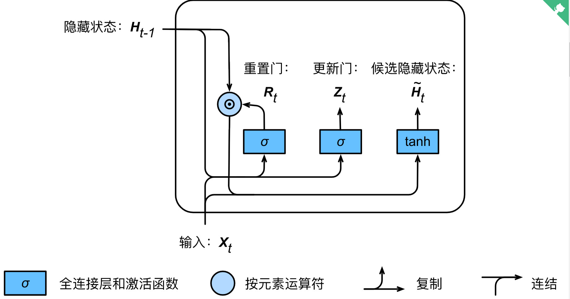
GRU门控单元
重置门和更新门的输入均为当前时间步的输入$X_t$与上一时间步的隐藏状态$H_{t-1}$, 激活函数都是sigmoid函数,因此它们的输出值域是$(0, 1)$,重置门的输出$R_t$用于得到候选隐藏状态,而更新门的输出$Z_t$用于在得到候选隐藏状态后确定该隐藏状态。
其中,候选隐藏状态计算为:
其中$\odot$是元素乘法, $R_t$在$(0, 1)$之间,因此重置门的作用可以看作用来筛选之前的历史信息$H_{t-1}$。
隐藏状态的计算为:
可见更新门在候选状态与上一时间步的状态作取舍,它的作用可以看作保存之前时刻的状态。
这样这两个的门的设计:重置门可理解为获取短期依赖关系,更新门可理解为获取长期依赖关系。
手动实现
1 | # 初始化参数 |
定义GRU计算
1 | def gru(inputs, state, params): |
直接使用之间的训练函数训练
1 | num_epochs, num_steps, batch_size, lr, clipping_theta = 160, 35, 32, 1e2, 1e-2 |
torch函数实现
直接调用GRU层即可
1 | lr = 1e-2 # 注意调整学习率 |
长短期记忆
长短期记忆(long short-term memory,LSTM)中包含三个门,输入门(input gate)、遗忘门(forget gate)和输出门(output gate),以及与隐藏状态形状相同的记忆细胞。
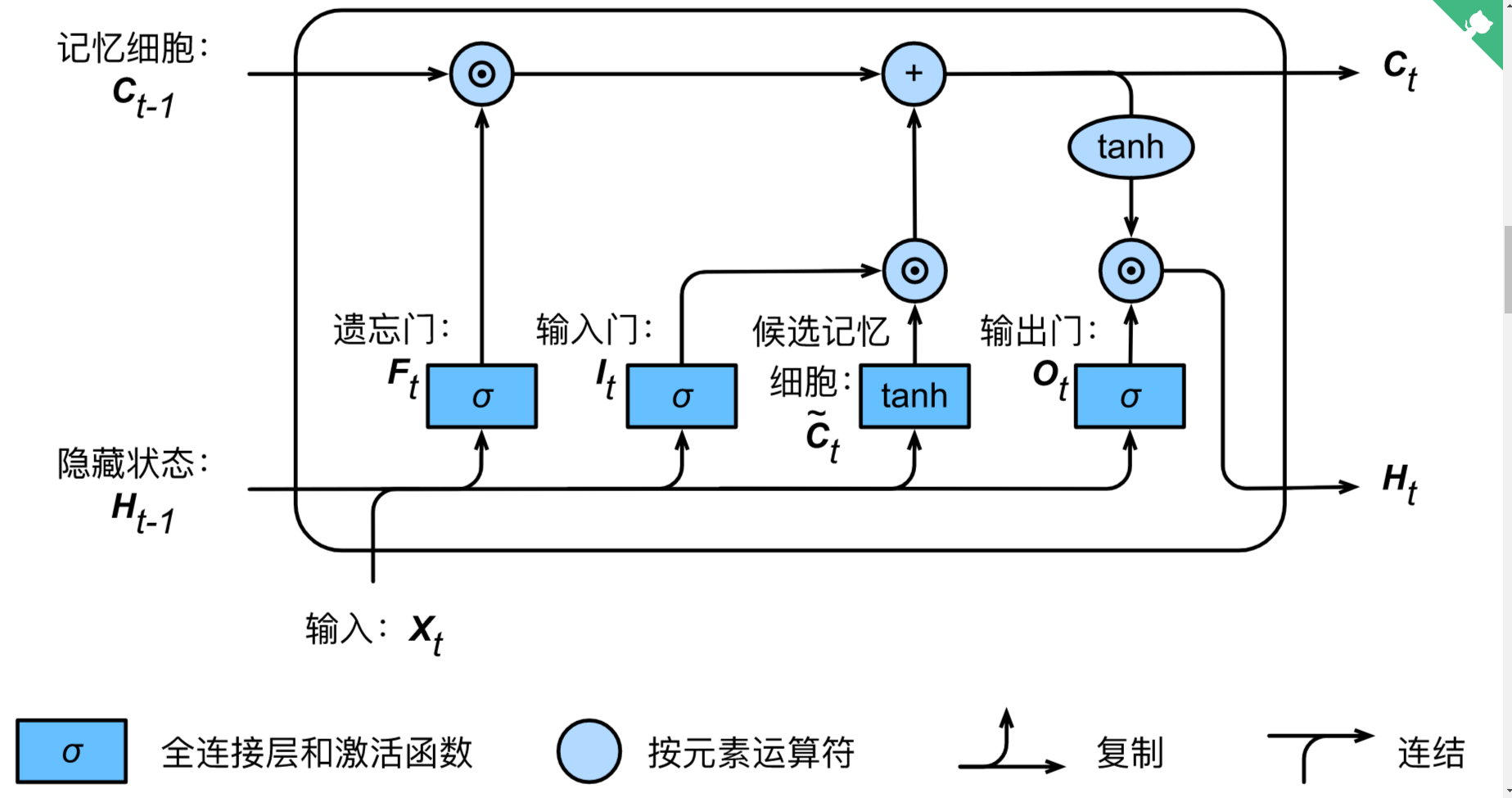
上图可以清晰的看出LSTM单元的计算过程,其中三个门控单元都是由上一时间步的隐藏状态和当前时间步的输入通过sigmoid函数得到,候选记忆细胞与它们的区别只是使用了tanh函数。然后通过这四个单元计算当前时间步的记忆细胞$C_t$和隐藏状态$H_t$。
手动实现
- 获取参数
1 | num_inputs, num_hiddens, num_outputs = vocab_size, 256, vocab_size |
- 初始化变量
LSTM会额外返回一个形状与隐藏状态相同的记忆细胞
1 | def init_lstm_state(batch_size, num_hiddens, device): |
- LSTM计算
其中记忆细胞$C_t$只在隐藏层间计算,不流动到输出层,输出层只计算隐藏状态。
1 | def lstm(inputs, state, params): |
- 训练
1 | num_epochs, num_steps, batch_size, lr, clipping_theta = 160, 35, 32, 1e2, 1e-2 |
torch函数实现
调用即可
1 | lr = 1e-2 # 注意调整学习率 |